
Sistema tekno-sozialak deritzonak osatzen dituzten zerbitzu teknologiko publiko eta globalak eskaintzeko gizartean elkarreragin egiten duten geruza ezberdinez osatutako azpiegiturak grafikoki irudikatu daitezke sare konplexuen bidez. Sare konplexuak sistema tekniko horien portaera modelatzeko oinarri gisa erabiltzen den paradigma matematikoa dira, eta haien portaera aurreikesteko gai dira. Sare konplexua ezaugarri topologiko ez hutsalak dituen grafo bat da, adierazle estatistikoen bidez ezaugarritu daitezkeenak, hala nola zentraltasun-neurri desberdinak eta komunitatearen detekzioa. Sare konplexuen aplikazioak garatu dira hainbat diziplinatan, hala nola Web-en, komunikazio-sareetan, garun-sareetan, sare biologikoetan, sare klimatikoetan, kirolean eta sare sozialetan. Artikulu honek intuizioz erakusten du sare konplexuen azpian dagoen teoria, baita datuetatik modelatzeko metodo desberdinak ere. Argibide gisa, aplikazioa sarbide irekiko software batekin aurkezten da, Euskal Herriko Unibertsitateko ikertzaileen artean aipamen bibliografikoen sare konplexu baten indukzio eta karakterizaziorako
Elements of complex networks
Elements of complex networks
Larrañaga, Pedro (1); P. Soloviev, Vicente (2)
- Filiazioa:
- Universidad Politécnica de Madrid. Artificial Intelligence Department. Campus de Montegancedo, s/n. 28660 - Boadilla del Monte, Madrid (1) pedro.larranaga@fi.upm.es; (2) vicente.perez.soloviev@upm.es
- Argitalpen urtea:
- 2023
- Argitalpen tokia:
- Donostia
- Ezaugarriak:
- BIBLID [0212-7016; eISSN: 2952-4180 (2023), 68, 2] - Recep: 2023-09-01; Accep: 2023-10-17
- ISSN:
- ISSN: 0212-7016; eISSN: 2952-4180
Erregistratu eta jaitsi Eusko Ikaskuntzaren argitalpenak
Erregistratuta nago. Kontura sartu
1. Introduction
A complex system is made up of several interconnected components whose interaction is capable of creating new properties, called emergent, unobservable when the system is seen from a disaggregated perspective. The human brain is an example of a complex system. In it, the observation of its basic elements, neurons --from any perspective, be it anatomical, electrophysiological or -omics and of their connections with other neurons does not allow us to get a precise idea of their global behavior.
A common way to graphically represent a complex system is by means of a graph (network) with non-trivial topological features, whose nodes denote the elements of the system and the edges indicate relationships between pairs of nodes. These types of graphs used to represent complex systems are called complex networks[1]. Complex network analysis aims to characterize these networks with a small number of meaningful and easily computable measures that have arisen in their applications in disciplines as diverse as the Web[2], communication networks[3], brain networks[4], biological networks[5], climate networks[6], sport[7], and social networks[8]. For reviews on complex networks, refer to[9] and[10].
Techno-social systems[11] are infrastructures made up of different technological layers that interoperate within society to provide global public services of a technological nature. Modern techno-social systems consist of large-scale physical (or cyber-physical) infrastructures embedded in a dense web of communication and computing infrastructures whose dynamics and evolution are defined and driven by human behavior. The prediction of the behavior of these systems is based on the mathematical modeling of the patterns underlying the data collected in the real world. Complex networks are the mathematical paradigm used as the basis for modeling the behavior of these techno-social systems.
This article seeks to introduce, intuitively, theoretical elements that serve to understand the behavior of complex networks from their mathematical modeling. The rest of the article is organized as follows. Section 1 introduces the main topological and structural characteristics of complex networks: degree distribution, centrality measures and community detection algorithms. Complex network models, such as Erdös-Renyi random networks, Watts-Strogatz model, and the Barabasi-Albert model are presented in Section 2. Section 3 illustrates some of the previous concepts with the application of an open access software to the induction and characterization of a complex network of bibliographic citations among researchers from a department at the Universidad del País Vasco/Euskal Herriko Unibertsitatea. Section 4 presents conclusions, and final remarks.
2. Topological and structural characteristics of complex networks
2.1. Centrality measures
The first works on graph centrality were developed in the 1940s at the Massachusetts Institute of Technology[12] in the sociological field, where centrality characteristics of a group and its efficiency in the development of different cooperative tasks were studied.
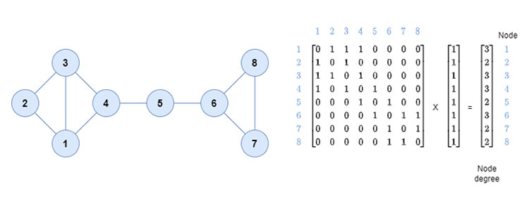
The idea of graph centrality is associated with three intuitively evident properties that the central elements of a network should verify[13]. The first property considers as central elements of a network those that have a greater degree of adjacency, that is, those that are related to a greater number of nodes. The node degree measures the number of its neighbors in the graph. It quantifies the node connectivity and is a local measure of centrality. Figure 1 shows an example in which node 5, which intuitively is more central than node 3, nevertheless has a lower node degree.
Figure 1. Illustration of the node degree vector computation by means of the adjacency matrix
A global measure of centrality of a node is the so-called eigenvector centrality. The eigenvector centrality[14] considers that the centrality of a node is proportional to the centrality of the nodes that are directly connected to it. The vector whose coordinates are the values of the eigenvector centralities of each one of the nodes turns out to be the eigenvector of the adjacency matrix of the graph corresponding to the eigenvalue of greatest absolute value. The way of calculating the eigenvector centrality presents similarities with the PageRank coefficient[15], famous for being the Google search engine and providing a ranking of importance to the web pages resulting from a given query. The PageRank coefficient of a given node is computed recursively from the PageRank coefficients of its neighboring nodes, normalized by their corresponding node degree. A damping coefficient influences the convergence of the Markov chain that models the stochastic process underlying such calculations.
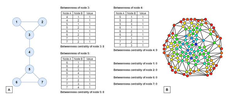
The second property establishes that the central elements of a network are those that belong to the largest possible number of shortest paths between any two nodes of the network. The intuition is that these nodes are good intermediaries because in order to take the shortest path from one node to another in the network, one would necessarily go through one of these nodes. Betweenness centrality[16] is a measure of centrality in a graph based on shortest paths. For every pair of vertices in a connected graph, there exists at least one shortest path between the vertices such that either the number of edges that the path passes through (for unweighted graphs) or the sum of the weights of the edges (for weighted graphs) is minimized. The betweenness centrality for each node is the quotient between the number of geodesics (shortest paths) between any two nodes that pass through the given node and the number of geodesics that join any two nodes, this number playing the role of normalizing constant. Betweenness centrality represents the degree to which nodes stand between each other. For example, in a telecommunications network, a node with higher betweenness centrality would have more control over the network, because more information will pass through that node. Figure 2 shows examples of betweenness centrality scores.
Figure 2. A. Betweenness centrality scores (without the normalizing constant) for a small graph.
B. An undirected graph colored based on the betweenness centrality of each vertex from least (red) to greatest (blue).
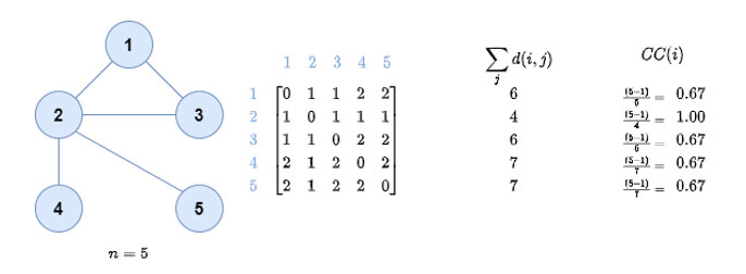
The third property is based on the fact that the central elements of a network are those that are closest to the rest of the nodes, that is, those that minimize the sum of geodesic distances to the rest of the nodes. The closeness centrality[17] of a node i, denoted as CC(i), measures how short the shortest paths are from node i to all the nodes and is defined as the normalized inverse of the sum of the geodesic distances in the graph: .png) is the number of nodes, and d(i,j) is the geodesic distance between i and j. Closeness centrality is a way of detecting nodes that are able to spread information very efficiently through a graph. See Figure 3 for an example.
is the number of nodes, and d(i,j) is the geodesic distance between i and j. Closeness centrality is a way of detecting nodes that are able to spread information very efficiently through a graph. See Figure 3 for an example.
Figure 3. Calculating the closeness centrality of nodes in a graph.
2.2. Community detection
Centrality measures are used for analyzing graphs whose nodes are elements of uniform collectives. However, sometimes the population under study contains inhomogeneous nodes. In this case, it is convenient to start the analysis with a detection of nodes with similar characteristics, to later carry out a more detailed analysis of each one of the groups.
The concept of community is based on those of intraclass density and extraclass density associated with a subset C of graphs nodes of the network. To calculate the intraclass density we need to calculate for each node of C the number of connections adjacent to said node that are in C. Adding over all nodes of C and normalizing by the total number of possible connections within C gives the intraclass density of C. The extraclass density will be obtained from the normalization of the total number of connections of each node of C with nodes outside of C. From these two concepts, it ensures that finding communities in graphs is reduced to finding subsets of graph nodes in which the difference between the intraclass density and the extraclass density is large enough.
Graph partition[18] is the reduction of a graph to a smaller graph by partitioning its set of nodes into mutually exclusive groups (the communities). Edges of the original graph that cross between the groups will produce edges in the partitioned graph. If the number of resulting edges is small compared to the original graph, then the partitioned graph may be better suited for analysis and problem-solving than the original. Graph partition problems fall under the category of NP-hard problems. For this reason, different combinatorial optimization heuristics have been applied (taboo search, ant colony optimization, genetic algorithms...) to obtain solutions to different instantiations of the graph partitioning problem.
The Kernighan–Lin algorithm[19] is a simple heuristic for finding graph partitions. The input to the algorithm is an undirected graph. The goal is to partition the node set into two disjoint subsets A and B of equal (or nearly equal) size, in a way that minimizes the sum of the weights of the subset of edges that cross from A to B. Instead, if the graph is unweighted, the goal is to minimize the number of crossing edges; this is equivalent to assigning weight one to each edge. The algorithm maintains and improves a partition, in each iteration using a greedy algorithm to pair up vertices of A with vertices of B, so that moving the paired vertices from one side of the partition to the other will improve the partition. After matching the vertices, it then performs a subset of the pairs chosen to have the best overall effect on the solution quality.
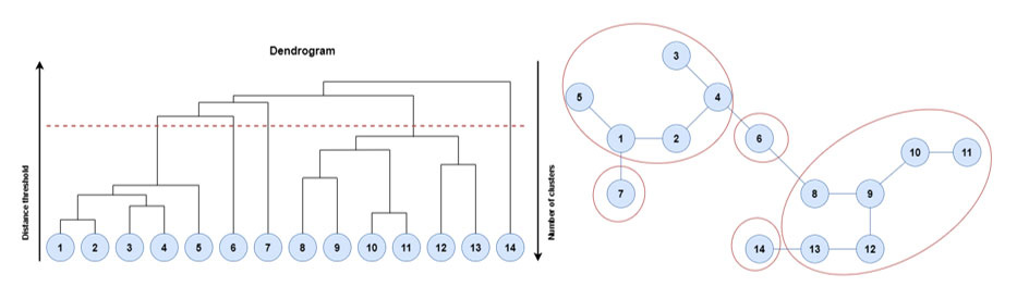
Community detection clustering algorithms are based on defining a distance, or alternatively a dissimilarity measure, between pairs of graph nodes to subsequently apply standard clustering methods, such as an agglomerative (or divisive) hierarchical clustering[20] or a partitional clustering[21]. Figure 4 shows the application of a hierarchical agglomerative algorithm for the detection of communities[22] in a graph with 14 nodes. The agglomerative hierarchical clustering algorithm starts with as many clusters as nodes, each singleton cluster with only one node. At each stage of the algorithm, the most similar pair of clusters is merged until all the objects belong to one cluster. There are different linkage strategies (single linkage, nearest neighbor linkage, average linkage, centroid linkage, or Ward’s method) for clusters merging depending on the definition of the dissimilarity between two clusters of nodes. A binary tree, called dendrogram, represents this process. The root node of the dendrogram contains all the graph nodes. The intermediate nodes describe how proximal the nodes are to each other. The height of the dendrogram represents the dissimilarity between each pair of nodes, or clusters of nodes, or between a node and a cluster of nodes. The clustering results can be output by cutting the dendrogram at different heights. The example of Figure 4 shows a solution for the community detection problem with five clusters or communities of nodes.
Figure 4. Example of a community detection result based on a hierarchical agglomerative algorithm
where the dendrogram where the threshold applied to the dendrogram has originated 5 clusters.
Partition clustering community detection algorithms[23] are based on the adaptation of partitional clustering methods to the problem of community detection in graphs. Although the best known partitional algorithm is K-means, other algorithms such as K-medians, K-modes, K-medoids, spectral clustering or affinity propagation can be used for this task.
3. Complex network models
There are several models of complex networks that can be used both for the random generation of said networks and to carry out hypothesis tests in which said models are set as null hypotheses to be tested from real world data. Three such complex network models will be introduced in this section.
3.1. Erdős-Rényi and Erdős-Rényi-Gilbert models
The Erdős-Rényi model[24] refers to one of two closely related models for generating random graphs or the evolution of a random network. These models are named after the Hungarian mathematicians Paul Erdős and Alfréd Rényi, who introduced one of the models in 1959. Edgar Gilbert introduced the other model, operating simultaneously and independently from Erdős and Rényi. In the model of Erdős and Rényi, all graphs on a fixed vertex set with a fixed number of edges are equally likely. In the model introduced by Gilbert, also called the Erdős–Rényi–Gilbert model[25], each edge has a fixed probability of being present or absent, independently of the other edges.
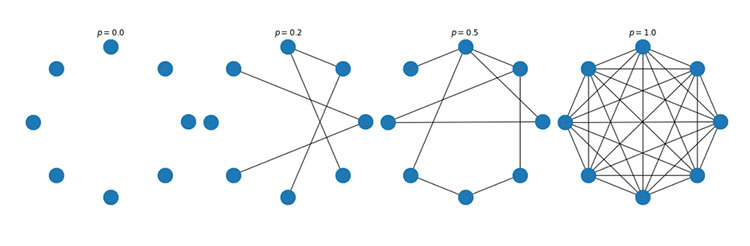
In the Erdős-Rényi model, denoted as G(n,m), a graph is chosen uniformly at random from the collection of all graphs which have n nodes and m edges. The nodes are considered to be labeled, meaning that graphs obtained from each other by permuting the vertices are considered to be distinct. For example, in the G(3,2) model, there are three two-edge graphs on three labeled vertices (one for each choice of the middle vertex in a two-edge path), and each of these three graphs is included with probability .png) . Figure 5 shows an example of a simulation of an Erdős-Rényi-Gilbert network.
. Figure 5 shows an example of a simulation of an Erdős-Rényi-Gilbert network.
Figure 5. An example of an Erdős-Rényi-Gilbert network with 8 nodes (top).
Topologies and node degree frequencies for different values of p (bottom).
The small-world experiment comprised several experiments conducted by Milgram, examining the average path length for social networks of people in the United States. The research was groundbreaking in that it suggested that human society is a small-world-type network characterized by short path-lengths. The experiments are often associated with the phrase "six degrees of separation", although Milgram did not use this term himself.
In this sense, an Erdős-Rényi network can be interpreted as a small-word network as we can see with the following example. Let consider one Erdős-Rényi network with a mean node degree given by k. If each node of said network communicates with each of its k neighbors, and this process is repeated r steps, we find that a total of krnodes have been connected. If k=r=10 we would have more nodes connected to each other than the total world population.
The Erdős–Rényi–Gilbert model is denoted as G(n,p). In it, a graph is constructed by connecting labeled nodes randomly. Each edge is included in the graph with probability p, independently from every other edge. Equivalently, the probability for generating each graph that has n nodes and m edges is .png) . The parameter p in this model can be thought of as a weighting function. As p increases from 0 to 1, the model becomes more and more likely to include graphs with more edges and less and less likely to include graphs with fewer edges. A graph in G(n,p) has on average
. The parameter p in this model can be thought of as a weighting function. As p increases from 0 to 1, the model becomes more and more likely to include graphs with more edges and less and less likely to include graphs with fewer edges. A graph in G(n,p) has on average .png) p edges. The distribution of the degree of any particular v vertex is binomial:
p edges. The distribution of the degree of any particular v vertex is binomial: .png)
.png) This probability distribution of the node degree converges when n and k → ∞ to a Poisson distribution of mean
This probability distribution of the node degree converges when n and k → ∞ to a Poisson distribution of mean .png) obtaining that
obtaining that .png) This convergence property of the node degree towards a Poisson distribution together with the lack of local clusters of nodes are two shortcomings of the Erdős–Rényi–Gilbert networks that invalidate them as models of a good number of situations in the real world.
This convergence property of the node degree towards a Poisson distribution together with the lack of local clusters of nodes are two shortcomings of the Erdős–Rényi–Gilbert networks that invalidate them as models of a good number of situations in the real world.
In percolation theory one examines a finite (or infinite) graph and removes edges randomly. Thus the Erdős–Rényi process can be seen as an unweighted link percolation on the complete graph, as the probability of removing each edge is the same. Alternative modeling, such as the Watts-Strogatz model and the Barabási-Albert model, are not percolation processes. Instead, they are rewiring and growth processes respectively (see below).
3.2. Watts-Strogatz model
The Watts–Strogatz model[26] is a random graph generation model that produces graphs with small-world properties, including short average path lengths and high clustering. Average path length, or average shortest path length is a concept in network topology that is defined as the average number of steps along the shortest paths for all possible pairs of network nodes. In graph theory, a clustering coefficient is a measure of the degree to which graph nodes tend to cluster together. Evidence suggests that in most real-world networks, and in particular social networks, nodes tend to create tightly knit groups characterized by a relatively high density of ties[27].
The Watts-Strogatz network generation process consists of two phases. In the first phase, we start with n ordered nodes and connect each one of them with an even k number of nodes, the .png) immediate predecessors and the following consecutive nodes. In a second phase, all the graph arcs are traversed, each one of them being eliminated with β probability. Then, one of its ends is reconnected with one of the other nodes, avoiding self-links or already existing arcs. If one of these two circumstances occurred, the arc in question would disappear.
immediate predecessors and the following consecutive nodes. In a second phase, all the graph arcs are traversed, each one of them being eliminated with β probability. Then, one of its ends is reconnected with one of the other nodes, avoiding self-links or already existing arcs. If one of these two circumstances occurred, the arc in question would disappear.
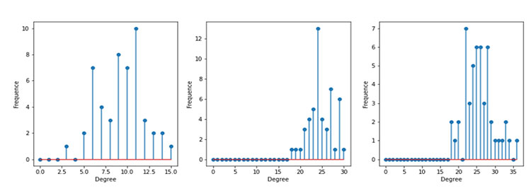
The topological properties of the resulting graph depend on β probability. In the case of β = 0, where the generated network is a regular network, the degree distribution is a Dirac Delta centered at 2k. If β =1, the graph is random and the nodal degree follows a Poisson distribution. Figure 6 shows the topology of a Watts-Strogatz network with 24 nodes with three different β values.
Figure 6. The Watts-Strogatz model. Different topologies depending on β values.
The major limitation of the model is that it produces an unrealistic degree distribution. In contrast, real networks are often scale-free networks (the degree distribution follows a power law) inhomogeneous in degree, having hubs and a scale-free degree distribution. Such networks are better described in that respect by the preferential attachment family of models, such as the Barabási–Albert model.
3.3. Barabási-Albert model
The Barabási–Albert model[28] is an algorithm for generating random scale-free networks using a preferential attachment mechanism. Many observed networks (at least approximately) fall into the class of scale-free networks. This means that they have scale-free degree distributions (that is, the probability of a node in the network having k connections to other nodes follows a power law: .png) , where γ is a parameter whose value is typically in the range 2 < γ < 3), while random graph models such as the Erdős–Rényi model and the Watts–Strogatz model do not exhibit power laws.
, where γ is a parameter whose value is typically in the range 2 < γ < 3), while random graph models such as the Erdős–Rényi model and the Watts–Strogatz model do not exhibit power laws.
The Barabási–Albert model incorporates two important general concepts: growth and preferential attachment. Both growth and preferential attachment exist widely in real networks. Growth means that the number of nodes in the network increases over time. Preferential attachment means that the more connected a node is, the more likely it is to receive new links. Nodes with a higher degree have a stronger ability to grab links added to the network.
Intuitively, the preferential attachment can be understood if we think in terms of social networks connecting people. Here a link from A to B means that person A "knows" or "is acquainted with" person B. Heavily linked nodes represent well-known people with lots of relations. When a newcomer enters the community, they are more likely to become acquainted with one of those more visible people rather than with a relative unknown. Preferential attachment is also sometimes called the Matthew effect, "the rich get richer". Several natural and human-made systems, including the Internet, the World Wide Web, citation networks, and some social networks are thought to be approximately scale-free and certainly contain few nodes (called hubs) with unusually high degree as compared to the other nodes of the network.
The only parameter in the Barabási–Albert model is m, a positive integer. The Barabási-Albert algorithm works as follows. The network starts with a set of .png) m randomly connected nodes. Note that 2 and the degree of each node in the initial network must be at least 1, otherwise the evolution of the network, as nodes are added, would cause them to remain completely disconnected from the network. New nodes are added to the network one by one. Each node is connected to m network nodes with a probability that is proportional to the number of links that the network nodes have, that is, the new nodes are linked preferably with the most connected nodes. Formally, the probability pi that a node connects to node i is
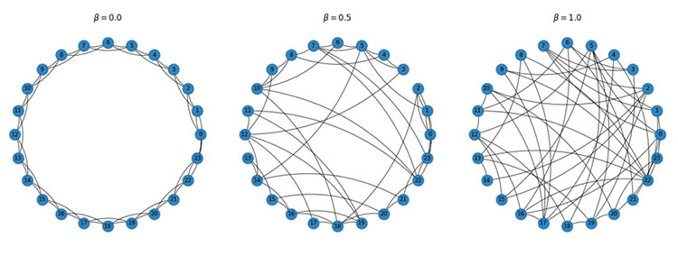
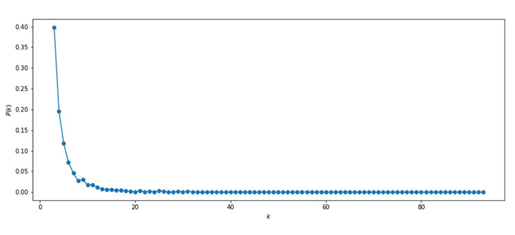
m randomly connected nodes. Note that 2 and the degree of each node in the initial network must be at least 1, otherwise the evolution of the network, as nodes are added, would cause them to remain completely disconnected from the network. New nodes are added to the network one by one. Each node is connected to m network nodes with a probability that is proportional to the number of links that the network nodes have, that is, the new nodes are linked preferably with the most connected nodes. Formally, the probability pi that a node connects to node i is .png) , where ki is the degree of node i. Nodes with a large number of connections (hubs) tend to quickly accumulate more links, while those with few links are rarely the source of new links. New nodes according to this algorithm are said to have a preference to be linked with the most requested nodes. This algorithm is based on the concept of preferential connection of the new nodes that join the network.The degree distribution resulting from the Barabási–Albert model is scale free, in particular, it is a power law of the form P(k) ~ k-3, as can be seen in Figure 7. An analytical result for its clustering coefficient was obtained in[29].
, where ki is the degree of node i. Nodes with a large number of connections (hubs) tend to quickly accumulate more links, while those with few links are rarely the source of new links. New nodes according to this algorithm are said to have a preference to be linked with the most requested nodes. This algorithm is based on the concept of preferential connection of the new nodes that join the network.The degree distribution resulting from the Barabási–Albert model is scale free, in particular, it is a power law of the form P(k) ~ k-3, as can be seen in Figure 7. An analytical result for its clustering coefficient was obtained in[29].
Figure 7. The power law distribution, P(k) ~ k-3, of the Barabási–Albert model with m=3 and n= 2000
4. Illustration example: A complex network of bibliographic citations
As an illustrative example, the graph of academic citations from a department at the Universidad del País Vasco/Euskal Herriko Unibertsitatea has been created. This graph is the result of data provided by Google Scholar and is shown in Figure 8. Each node of said graph corresponds to a member of the analyzed department, while an edge between two members indicates the existence of a scientific work of which both researchers are co-authors. No weights have been assigned to the edges, even if it could have been done taking into account the number of works jointly published by both researchers. No restrictions have been imposed on the period of time analyzed. Therefore, there may be edges between researchers who jointly published many years ago, but who currently do not collaborate scientifically. These last two issues undoubtedly limit the results of the analysis. On the other hand, the analysis has been carried out using exclusively the concepts introduced in Section 1.
Figure 8. Graph representing academic bibliographic co-citations among the 28 members from
a department at the Universidad del País Vasco/Euskal Herriko Unibertsitatea.
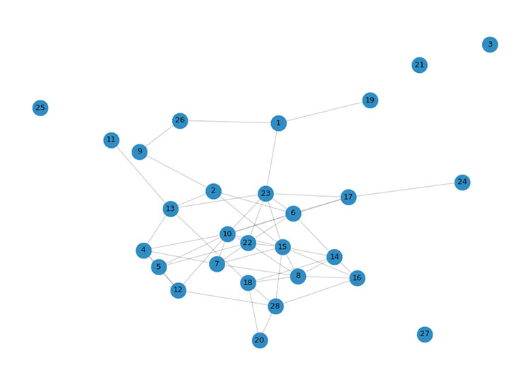
Table 1 shows the values of three centrality measures calculated for a department member from the graph in Figure 8. Table 1 illustrates that the node degree varies from 0 to 9. The 0-s correspond to the four nodes without edges, while the highest value (node degree = 9) is achieved by two members recognized for being directors of research groups. In the third column of Table 1 we can read the betweenness centrality values of each node without normalizing. In general, these values show a high correlation with their corresponding node degree values. There are striking cases, such as those of nodes 1 and 10, with similar values in terms of betweenness centrality but very different values in node degree. Nodes 22 and 23 also stand out with the same value of node degree and very different values in betweenness centrality. The fourth column of Table 1 contains the closeness centrality values for each node. These values show a stronger correlation with node degree than with betweenness centrality. It is worth noting the high value of closeness centrality in node 13 when compared to its node degree.
Table 1. Centrality measures for the graph nodes in Figure 8
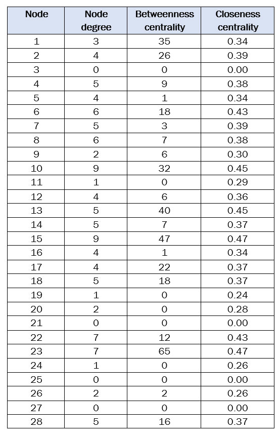
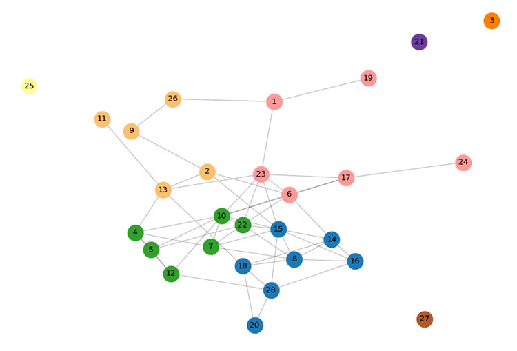
Figure 9 shows the dendrogram that represents the hierarchical agglomerative clustering of the 28 nodes in Figure 8. The red dashed line has been used as a threshold to obtain the 8 clusters (see Figure 10), each with a different color. Four of the clusters have a single member. It has been confirmed that the other four clusters correspond to the four existing research groups within the department, indicating the validity of this method for detecting communities in complex networks.
Figure 9. Hierarchical agglomerative clustering of the 28 nodes in Figure 8
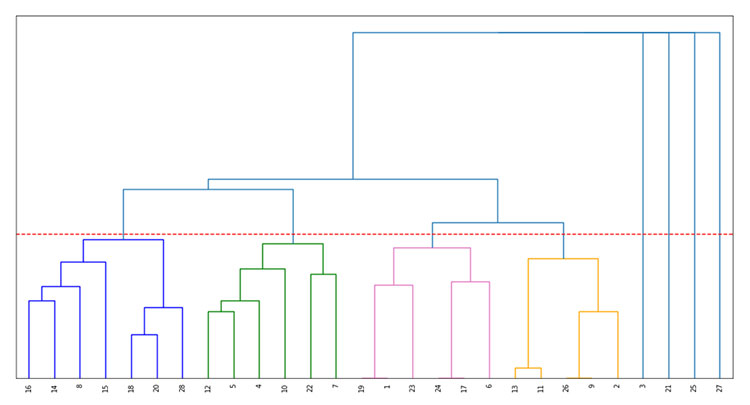
Figure 10. Eight clusters resulting from the detection of existing communities in the graph illustrated
in Figure 8 and the hierarchical agglomerative clustering method in Figure 9
5. Conclusions and final remarks
In this article some elements of complex networks have been presented, which constitute a useful paradigm to quantitatively analyze techno-social systems. Basic topological and structural features have been introduced in complex networks such as graph centrality, node degree, eigenvector centrality, or the Page-Rank coefficient. The concepts of betweenness, centrality and closeness centrality have been illustrated with explanatory examples. Some community detection algorithms have been explained, such as the Kernighan-Lin algorithm and various community detection clustering algorithms, both based on hierarchical agglomerative algorithms and partitional clustering methods. Complex network models commonly used in the literature have been included: the Erdős-Rényi model, as a generator of small-word networks and an example of a percolation process; the Watts-Strogatz model, as a graph generator with small-word properties, short average path lengths and high clustering; finally, the Barabási-Albert model from which random scale-free networks can be obtained using a preferential mechanism. An example of application in the field of academic co-citations in a department of the Universidad del País Vasco/Euskal Herriko Unibertsitatea has been analyzed, using the elements previously introduced.
It is out of the scope of this work to provide a list of additional methods and algorithms with the same objective as those already introduced. We believe that the reader can benefit to a greater extent from some reflections in relation to more relevant and current research aspects on this topic.
A fundamental concern refers to the statistical modeling from data, trying to find the most likelihood complex network structure. In this sense, a current trend is the adaptation of the modeling methods of probabilistic graphical models (Markov networks and Bayesian networks) that have reached a high level of development within statistical machine learning. Another aspect of interest in the use of probabilistic graphical models is that they can be applied to carry out future predictions using temporal versions (temporal Bayesian networks, dynamic Bayesian networks or continuous time Bayesian networks). The existence of exact evidence propagation procedures that allow for different kinds of probabilistic reasoning (predictive, diagnostic, intercausal, abductive, counterfactual, ...) is another argument in favor of probabilistic graphical models.
A further novel topic concerns spatial networks. While most of the early works on complex networks have focused on the characterization of their topological properties, the spatial aspect has received less attention, when not neglected at all. However, it is not surprising that the topology could be constrained by the geographical embedding.
Many real networks are interrelated with each other and cannot be analyzed in isolation. In this sense, in recent years the study of networks of real networks has begun, what is known as multiplex networks. An example very easy to understand is the transportation network that includes, for instance, the airport network, the highway network and the metro network. In the case of the airport network, it is usually modeled as a single network where the nodes are the airports and the edges are the direct flights between airports. However, a better representation would be to consider a multiplex network made up of many networks, each of which would correspond to a particular airline, where each node would again be the airport and each edge would correspond to the direct flights between airports carried out by that company. It may happen that each of these networks has the same set of nodes but different edges, since not all airlines have flights between the same airports. The study of this multiplex network has much importance, for example, to re-accommodate passengers who have missed their flights on a flight from another company due to the high economic costs involved. In general, complex infrastructures are totally interdependent so that a small failure in a network can cause a cascade of failures in all interdependent networks.
The development of complex networks that include methodologies from probabilistic graphical models, spatial statistics and multiplex networks will enable the modelling of more complex situations already present in the real world. It will also provide tools to carry out probabilistic reasoning, significantly improving the applied research obtained from complex networks. However, for this to occur, a good number of limitations derived from the current scarce methodological development of probabilistic graphical models at the level of spatiality and in scenarios as interrelated as multiplex networks should be overcome.
[1] Newman, M. (2003). The structure and function of complex networks. SIAM Review, 45 (2), 167-256.
[2] Scharnhost, A. (2006). Complex networks and the Web: Insights from nonlinear physics. Journal of Computer-Mediated Communication, 8 (4), JCMC845.
[3] Niazi, M.A. (2019). Modeling and Simulation of Complex Communication Networks. IET Digital Library.
[4] Rubinov, E., Sporns, O. (2010) Complex network measures of brain connectivity: Uses and interpretations. NeuroImage, 52(3), 1059-1069.
[5] Jeong, H., Tombor, B., Albert, R., Oltvai, Z. N., Barabási, A. L. (2000). The large-scale organization of metabolic networks. Nature, 407(6804), 651-654.
[6] Donges, J.F., Zou, Y., Marwan, N., Kurths, J. (2009). Complex networks in climate dynamics. The European Physical Journal Special Topics, 174, 157-179.
[7] Gong, B., Zhou, C., Gómez, M.A., Buldú, J.M. (2023). Identifiability of Chinese football teams: A complex networks approach. Chaos, Solitons and Fractals, 166.
[8] Vega-Redondo., F. (2007). Complex Social Networks. Cambridge University Press.
[9] Walker, G.H., Stanton, N.A., Salmon, P.M., Jenkins, D.P. (2008). A review of sociotechnical systems theory: A classic concept for new command and control paradigms. Theoretical Issues in Ergonomic Science, 9(6), 479-499.
[10] Boccalettia, S., Latorab, V., Morenod, Y., Chavezf , M., Hwanga, D.U. (2006). Complex networks: Structure and dynamics. Physics Reports, 424, 175-308.
[11] Sousa da Mata, A., (2020). Complex networks: A mini-review. Brazilian Journal of Physics, 50, 658-672.
[12] Bavelas, A., Barret, D. (1945). An Experimental Approach to Organizational Communication. Department of Economics and Social Sciences. Massachusetts Institute of Technology.
[13] Freeman, L.C. (1979). Centrality in social networks: Conceptual clarification. Social Networks, 1, 215-239.
[14] Langville, A., Meyer, C. (2006). Google's PageRank and Beyond: The Science of Search Engine Rankings. Princeton University Press.
[15] Page, L., Brin, S., Motwani, R., Winograd, T. (1998) The PageRank Citation Ranking: Bringing Order to the Web. Technical Report SIDL-WP-1999-0120, Stanford Digital Library Technologies Project.
[16] Brandes, U. (2001). A faster algorithm for betweenness centrality. The Journal of Mathematical Sociology, 25(2), 163-177.
[17] Beauchamp, M. A. (1965). An improved index of centrality. Systems Research and Behavioral Science, 10 (2), 161-163.
[18] Wu, S., Hou, J. (2023). Graph partitioning: An updated survey. AKCE International Journal of Graphs and Combinatorics, 20(1), 9-19.
[19] Kernighan, B. W., Lin, S. (1970). An efficient heuristic procedure for partitioning graphs. Bell System Technical Journal, 49, 291–307.
[20] Florek, K., Lukaszewicz, J., Perkal, H., Steinhaus, H., Zubrzycki S. (1951). Sur la liason et la division des points d’un ensemble fini. Colloquium Mathematicum, 2, 282-285.
[21] MacQueen, J. (1967). Some methods for classification and analysis of multivariate observations. Proceedings of the 5th Berkeley Symposium on Mathematical Statistics and Probability, 281-297.
[22] Zhang, S., Ning, X.M., Zhang, X.S. (2007). Graph kernels, hierarchical clustering, and network community structure: experiments and comparative analysis. The European Physical Journal B 57(1), 67-74.
[23] Alguliev, R.M., Aliguliyev, R.M., Ganjaliyev, F.S. (2013). Partition clustering-based method for detecting community structures in weighted social networks. International Journal of Information Processing and Management, 4, 60-72.
[24] Erdős, P., Rényi, A. (1959). On random graphs. I. Publicationes Mathematicae 6, 290–297.
[25] Gilbert, E.N. (1959). Random graphs. Annals of Mathematical Statistics, 30(4), 1141–1144.
[26] Watts, D. J., Strogatz, S. H. (1998). Collective dynamics of 'small-world' networks. Nature, 393, 440-442.
[27] Holland, P. W., Leinhardt, S. (1971). Transitivity in structural models of small groups. Comparative Group Studies, 2(2), 107–124.
[28] Barabási, A.L., Albert, R. (1999). Emergence of scaling in random networks. Science 286, 509-512.
[29] Klemm, K., Eguíluz, V. C. (2002). Growing scale-free networks with small-world behavior. Physical Review E, 65 (5): 057102.
PARTEKATU